Inter 1st Year Maths 1B Applications of Derivatives Formulas

Use these Inter 1st Year Maths 1B Formulas PDF Chapter 10 Applications of Derivatives to solve questions creatively.

Intermediate 1st Year Maths 1B Applications of Derivatives Formulas

→ Error in y = Δy = f(x + Δx) – f(x)

→ Differential in y = dy = f’ (x) Δx

→ Relative error in y = \(\frac{\Delta y}{y}\)

→ Percentage error in y = \(\frac{\Delta y}{y}\) × 100

Circle:
if’ r’ is the radius, x is the diameter, p is the perimeter (circumference) and A is the area of a circle then

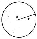
• A = πr or A = \(\frac{\pi x^{2}}{4}\)
• x = 2r
• p = 2πr (or) p = πx

Sector :
If ‘r’ is the radius, l is the length of arc and ‘θ’ is the angle then

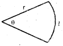
• Area = A = \(\frac{1}{2}\)r (or) A = \(\frac{1}{2}\)r²θ
• Perimeter = p = l + 2r (or) p = r (θ + 2)
• l = rθ

Cylinder :
If ‘r’ is the radius, h is the height then

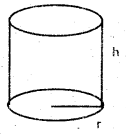
• Lateral surface area = 2πrh
• Total surface area = S = 2πrh + 2πr²
• Volume = V = πr²h

Cone:

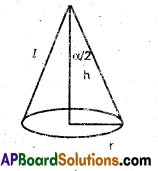
r is base radius, h is the height, ‘l’ is the slant height, a is the vertical angle then

• l² = r² + h²
• tan \(\frac{\alpha}{2}=\frac{r}{h}\)
• Lateral surface area = πrl (or) πr\(\sqrt{r^{2}+h^{2}}\)
• Total surface area = S = πrl + πr² (or) S = πr \(\sqrt{r^{2}+h^{2}}\) + πr²
• Volume = V = \(\frac{1}{3}\)πr²h

Simple pendulum:
If ‘l’ is the length, T is the period of oscillation of a simple pendulum and g is the acceleration due to gravity then T = 2π\(\sqrt{\frac{l}{g}}\)

Sphere :
‘r’ is the radius,

• Surface area = S = 4πr
• Volume = V = \(\frac{4}{3}\) πr³

Cube :
Let ‘x’ is the side

• Surface area = S = 6x²
• Volume = V = x³

→ Slope of the tangent = f'(x)

→ Equation of the tangent is (a, b) is y – b = f'(a) (x – a)

→ Equation of the normal at (a, b) is y – b = –\(\frac{1}{f^{\prime}(a)}\) (x – a)

→ Length of the tangent = \(\left|\frac{f(a) \sqrt{1+\left(f^{\prime}(a)\right)^{2}}}{f^{\prime}(a)}\right|\)

→ Length of the normal = \(\left|f(a) \sqrt{1+\left[f^{*}(a)\right]^{2}}\right|\)

→ Length of the sub-tangent = \(\left|\frac{f(a)}{f^{\prime}(a)}\right|\)

→ Length of the sub-normal = |f(a).f'(a)|

Angle between the curves is tan Φ = \(\left|\frac{m_{1}-m_{2}}{1+m_{1} m_{2}}\right|\)

→ If m₁ = m₂, the curves touch each other and have a common tangent

→ If m₁m₂ = -1, the curves cut orthogonally

→ If a particle starts from a fixed point and moves a distance ‘s’ along a straight line during time ‘t’, then
v = velocity of the particle at the time t = \(\frac{\mathrm{ds}}{\mathrm{dt}}\)
a = acceleration of the particle at the time t = \(\frac{\mathrm{d}^{2} \mathrm{~s}}{\mathrm{dt}^{2}}\) = v\(\frac{\mathrm{dv}}{\mathrm{ds}}\)

• If v > 0, then the particle is moving away from the straight point.
• If v < 0, then the particle is moving towards the straight point.
• If v = 0, then the particle comes to rest.

→ Let O be a fixed in a plane and OX be a fixed ray in the same plane. Let P be the position of a particle on a curve C, at time ‘f and ∠XOP = θ.

• ω = Angular velocity of the particle around ‘O’ = \(\frac{\mathrm{d} \theta}{\mathrm{dt}}\)
• Angular acceleration of the particle around ‘O’ = \(\frac{\mathrm{d}^{2} \theta}{\mathrm{dt}{ }^{2}}\) (Where θ is in radian measure).

→ Increasing and Decreasing functions: A function f(x) is

• Increasing if f'(x) > 0
• Decreasing if f'(x) < 0′
• f(x) is stationary if f’ (x) = 0

→ A function f(x) has local maxima or local minima only at stationary points.

• f(x) has local maximum of f’(x) = 0, f”(x) < 0 f(x) has local minimum if
• f’(x) = 0, f”(x) > 0
  Absolute maximum = max. {local maxima}
  Absolute minimum = Min {local minima}.

Tangent To A Curve:
Definition :
Let y = f(x) be a curve and P be a point on the curve. If Q is a point on the curve other than P, then PQ is called a secant line of the curve. If the secant line \(\overline{P Q}\) approaches the same limiting position as Q approaches P along the curve from either side then the limiting position is called the tangent line to the curve at the point P. The point P is called the point of contact of the tangent line to the curve.

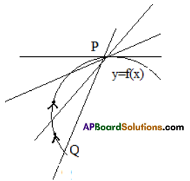
The tangent at a point to a curve, if it exists, is unique. Therefore, there exists at most one tangent at a point to a curve.

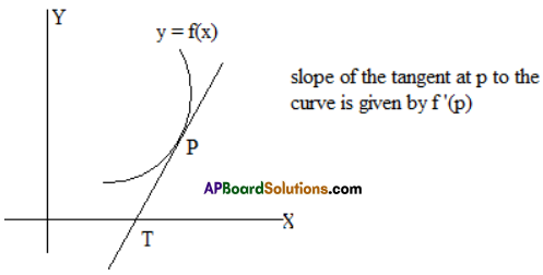
Geometrical Interpretation Of Derivative:
Let P be a point on the curve y = f(x). Then the slope of the tangent to the curve at P is equal to \(\left(\frac{d y}{d x}\right)_{P}\) i.e., (f'(x))_p

Gradent The slope of the tangent at a point to a curve is called the gradient of the curve at that point.

The gradient of the curve y = f(x) at P is \(\left(\frac{d y}{d x}\right)_{P}\)

Note:

• If \(\left(\frac{d y}{d x}\right)_{P}\) = o then the tangent to the curve at P is parallel to the x – axis. The tangent, in this case, is called a horizontal tangent.
• If \(\left(\frac{d y}{d x}\right)_{P}\) = +∞ or -∞ i.e., if \(\left(\frac{d y}{d x}\right)_{P}\) = 0 then the tangent to the curve at P is perpendicular to x – axis. The tangent, in this case, is called a vertical tangent.
• If \(\left(\frac{d y}{d x}\right)_{P}\) does not exist then there exists no tangent to the curve at P.

Equation of Tangent:
The equation of the tangent at the point P(x₁, y₁) to the curve y = f(x) is y – y₁ = m(x – x₁)
where m = \(\left(\frac{d y}{d x}\right)_{P}\)

Note:

• x – intercept of the tangent = x₁ – \(\frac{y_{1}}{m}\) = x₁ – y₁m
• y – intercept of the tangent = y₁ – mx₁ = y₁ – x₁m

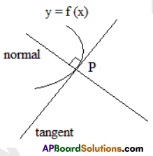
Normal To A Curve
Let P be a point in the curve y = f(x). The line passing through P and perpendicular to the tangent at P to the curve is called the normal to the curve at P.

The slope of the normal to the curve y = f(x) at P is m’ = \(\frac{1}{m}=-\left(\frac{d x}{d y}\right)_{P}\) where m = \(\left(\frac{d y}{d x}\right)_{P}\) ≠ 0

The equation of the normal at p(x₁, y₁) to the curve y = f(x) is
y – y₁ = \(\frac{-1}{m}\)(x – x₁) where m = \(\left(\frac{d y}{d x}\right)_{P}\)
i.e., y – y₁ = \(\left(\frac{d y}{d x}\right)_{P}\)(x – x₁)

Infinitesimals:
Let x be a finite variable quantity and be a minute change in x. Such a quanitity , which is very small when compared to x and which is smaller than any pre-assigned small quantity, is called an infinitesimal or an infinitesimal of first order. If δX is an infinitesimal then (δX)² , (δX)³ , …….. are called infinitesimals respectively of 2nd order, 3rd order….

If A is a finite quantity and is an infinitesimal then A. δX , A. (δX)² , A. (δX)³, ………. are also infinitesimals and they are infinitesimals respectively of first order, second order, third order
Definition: A quantity α = α(x) is called an infinitesimal as x → a if \({Lt}_{x \rightarrow a} α(x)\) = 0

Theorem:
Let y = f (x) be a differentiable function at x and be a small change in x. Then f'(x) and \(\frac{δ}{δ x}\) differ by an infinitesimal G(δx) as δx → 0 , where δy = f (x + δx) – f (x).

Differential
Definition: If y = f (x) is a differentiable function of x then f ’(x)S is called the differential of f. It is denoted by df or dy.
dy = f'(x)δx or df = f'(x)δx.
Note: δf = df i.e., error in f is approximately equal to differential of f

Approximations:
We have δf = f (x + δx) – f (x) ………………(1)
⇒ df ≅ f (x + δx) – f (x)
⇒ f’ (x)δx ≅ f (x + δx) – f (x)
⇒ f (x + δx) ≅ f (x) + f’ (x)δx
If we know the value of f at a point x, then the approximate value of f at a very nearby point x + δX can be calculated with the help of above formula.

Errors
Definition: Let y=f(x) be a function defined in a nbd of a point x. Let δx be a small change in x and δy be the corresponding change in y.
If δx is considered as an error in x, then

• δf is called the absolute error or error in y,
• \(\frac{δy}{y}\) is called the relative error (or proportionate error) in y,
  \(\frac{δy}{y}\) × 100 is called the percentage error in y corresponding to the error ox in x.

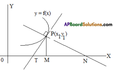
Lengths Of Tangent, Normal, Subtangent And Sub Normal
Definition :
Let y = f (x) be a differentiable curve and P be a point on the curve.
Let the tangent and normal at P to the curve meet the x – axis in T and N respectively. Let M be the projection of P on the x – axis. Then
(i) PT is called the length of the tangent,
(ii) PN is called the length of the normal
(iii) TM is called the length of the subtangent,
(iv) MN is called and length of the subnormal at the point P.

Let P(x₁, y₁) be a point on the curve y = f (x). Then

• The length of the tangent to the curve at P is \(\left|\frac{y_{1}}{m} \sqrt{1+m^{2}}\right|\)
• the length of the normal to the curve at P is |y₁\(\sqrt{1+m^{2}}\)|
• the length of the subtangent to the curve at P is \(\left|\frac{y_{1}}{m}\right|\)
  the length of the subnormal to the curve at P is |y₁m| where m = \(\left(\frac{d y}{d x}\right)_{P}\)

Angle between two curves:
If two curves intersect at P then the angle between the tangents to the curves at P is called the angle between the curves at P.

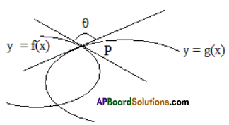
Angle between the curves:
Let y = f (x) and y = g(x) be two differentiable curves intersecting at a point P. Let m₁ = [ f'(x)]_P , m₂ = [g'(x)]_P be the slopes of the tangents to the curves at P. If θ is the acute angle between the curves at P then tan θ = \(\left|\frac{m_{1}-m_{2}}{1+m_{1} m_{2}}\right|\)

Note:

• If m₁ = m₂ then θ = 0. In this case the two curves touch each other at P. Hence the curves have a common tangent and a common normal at P.
• If m₁m₂ = -1then θ = \(\frac{\pi}{2}\). In this case the curves cut each other orthogonally at P.
• If m₁ = 0 and \(\frac{1}{m_{2}}\) = 0 then the tangents to the curves are parallel to the coordinate axes.
• Therefore the angle between the curves is θ = \(\frac{\pi}{2}\)

Rate of Changes:
Let y = f(x) be defined on an interval (a,b). let δy be change in y corresponding to a change δx in x.
Then , \(\frac{\Delta y}{\Delta x}\) is called average rate of change of y. if \(\underset{δx \rightarrow 0}{L t} \frac{\Delta y}{\Delta x}\) exists finitely, the this limit (i.e., \(\frac{d y}{d x}\)) is called rate of change of y with respect to x .

Note:
\(\left(\frac{d y}{d x}\right)_{a t \mathrm{x}=\mathrm{c}}\) represents the rate of change of y with respect to x at x = c.

Rectilinear Motion:
Let a particle start at a point O on a line L and move along the line. After a time of t units, let the particle be at P and OP = s. Since s is dependent on time t, we write s=s(t). s is called the displacement of the particle during time t.
The rate of change of displacement s is called the velocity of the particle and it is denoted by v = \(\frac{d s}{d t}\).
The rate of change of velocity is called acceleration. It is denoted by a.
a = \(\frac{d v}{d t}=\frac{d}{d t}\left(\frac{d s}{d t}\right)=\frac{d^{2} s}{d t^{2}}\)

Angular Velocity:
At time t, let P be the position of a moving point, Q be the position of the point after an interval δt. Let ∠xop = 6 and ∠POQ = δθ

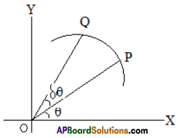
The angular velocity of P at O is\(\underset{x \rightarrow 0}{L t} \frac{δθ}{δt}=\frac{dθ}{d t}\)
Angular velocity w\(\frac{d \theta}{d t}\)
The angular acceleration of P at O is \(\frac{d \omega}{d t}=\frac{d}{d t}\left(\frac{d \theta}{d t}\right)=\frac{d^{2} \theta}{d t^{2}}\)

Maxima And Minima
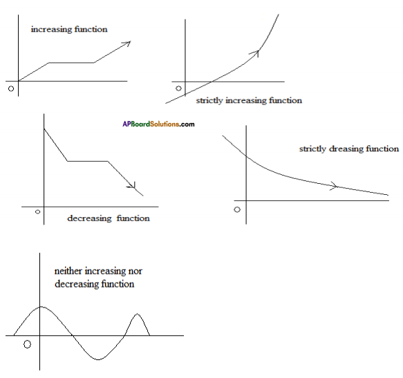
Monotonic Functions Over An Internal
Definition: A function f :[a, b] → R is said to be
(i) Monotonically increasing (or non – decreasing) on [a, b] if x₁ < x₂ ⇒ f (x₁) ≤ f (x₂) ∀ x₁,x₂ ∈ [a, b]
(ii) Monotonically decreasing (or non – increasing) on [a, b] if x₁ < x₂ ⇒ (x₁) ≥ f (x₂) ∀ x₁,x₂ ∈ [a, b]
(iii) strictly increasing on [a, b] if x₁ < x₂ ⇒ (x₁) < f (x₂) ∀ x₁,x₂ ∈ [a, b]
(iv) strictly decreasing on [a, b] if x₁ < x₂ ⇒ (x₁) > f (x₂) ∀ x₁,x₂ ∈ [a, b]
(v) a monotonic function on [a, b] if f is either monotonically increasing or monotonically decreasing on [a, b].

Theorem:
Let f be a function defined in a nbd of a point a and f be differentiable at a. Then

• f'(a) > 0 ⇒ f is locally increasing at a.
• f >(a) < 0 ⇒ f is locally decreasing at a. Note: Let f be continuous on [a, b] and differentiable on (a, b). Then (i) f'(x) ≥ 0 ∀ x ∈ (a,b) ⇒ f (x) is increasing on [a, b]. (ii) f'(x) ≤ 0 ∀ x ∈ (a,b) ⇒ f (x) is decreasing on [a, b].
• f'(x) > 0 ∀ x ∈ (a,b) ⇒ f (x) is strictly increasing on [a, b].
• f'(x) < 0 ∀ x ∈ (a,b) ⇒ f (x) is strictly decreasing on [a, b].
• f'(x) = 0 ∀ x ∈ (a,b) ⇒ f (x) is a constant function on [a,b].

Greatest And Least Values
Definition: Let f be a function defined on a set A and l ∈ f (A). Then l is said to be
(i) the maximum value or the greatest value of f in A if f (x) ≤ l ∀ x ∈ A .
(ii) the minimum value or the least value of f in A if f (x ) ≥ l ∀ x ∈ A

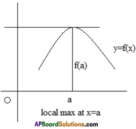
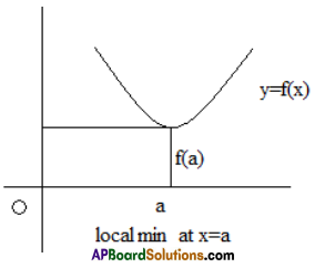
Local Maximum And Local Minimum Values
Let f be a function defined in a nbd of a point ‘a’ then f is said to have
(i)a local maximum (value) or a relative maximum at a if ∃ a δ > 0 such that f (x) < f (a) ∀ x ∈ (a – δ, a) ∪ (a, a + δ) . In this case a is called a point of local maximum of f and f (a) is its local maximum value.

(ii) a local minimum (value) or relative minimum at a if 3 a 5> 0 such that f (x) > f (a) ∀ x ∈ (a – δ, a) ∪ (a, a + δ). In this case a is called a point of local minimum and f (a) is its local minimum value.

Theorem:
Let f be a differentiable function in a nbd of a point a. The necessary condition for f to have local maximum or local minimum at a is f ‘(a) = 0.

First Derivative Test
Let f be a differentiable function in a nbd of a point a and f'(a) = 0. Then

• f (x) has a relative maximum at x =a if ∃ a δ > 0 such that
  x ∈ (a – δ, a) ⇒ f'(x) > 0 and x ∈ (a, a + δ) ⇒ f'(x) < 0 .
• f(x) has a relative minimum at x= a if 3 a 8> 0 such that
  x ∈ (a – δ, a) ⇒ f'(x) < 0 and x ∈ (a, a +δ) ⇒ f'(x) < 0 .
• f (x) has neither a relative maximum nor a minimum at x=a if f'(x) has the same sign for all x ∈ (a – δ, a) ∪ (a, a + δ) .

Second Derivative Test
Let f (x) be a differentiable function in a nbd of a point ‘a’ and let f”(a) exist.

• If f'(a) = 0 and f”(a) < 0 then f (x) has a relative maximum at f (x) and the maximum value at a is f (a).
• If f'(a) = 0 and f”(a) > 0 then f (x) has a relative minimum at f (x) and the minimum value at a is f (a).

Absolute Maxima And Absolute Minima
Let f be a function defined on [a, b]. Then

• Absolute maximum of f on [a, b] = Max.{ f (a), f (b) and all relative maximum values of f in (a, b)}.
• Absolute minimum of f on [a, b] = Min.{ f (a), f (b) and all relative minimum values of f in (a,b)}.

Note :

• maximum and minimum values are called extrimities.
• If f'(a) = 0 , then f is said to be stationary at a and f(a) is called the stationary value of f. and (a, f(a)) is called a stationary point of f.

Mean Value Theorems
Rolle’sTheorem :If a function f : [a, b] → R is such that

• It is continuous on [a, b]
• It is derivable on (a, b) and i
• f(a) = f(b) then there exists at least one C ∈ (a,b) such that f ‘(C) = 0.

Lagrange’s mean -value theorem or first mean – value theorem :
If a function f : [a, b] → R is such that

• It is continuous on [a, b].
• It is derivable on (a, b) then there exists at least one C ∈ (a,b) such that \(\frac{f(b)-f(a)}{b-a}\) = f ‘(C)