Inter 1st Year Maths 1B Limits and Continuity Formulas

Use these Inter 1st Year Maths 1B Formulas PDF Chapter 8 Limits and Continuity to solve questions creatively.

Intermediate 1st Year Maths 1B Limits and Continuity Formulas

Right Limit :
Suppose f is defined on (a, b) and Z ∈ R. Given ε < 0 , there exists δ > 0 such that a < x < a + δ => |f(x) – l| < ε, then l is said to be the right limit of’ f’ at ‘a’.
It is denoted by \({Lt}_{x \rightarrow a+} f(x)\)f(x) = l

Left Limit :
Suppose ‘ f’ is defined on (a, b) and Z e R. Given e > 0, there exists δ > 0 such that a – δ < x < a ⇒ |f(x) – l| < ε, then l is said to be the left limit of’ f’ at ’a’ and is denoted by \({Lt}_{x \rightarrow a-} \dot{f(x)}\) = l

Suppose f is defined in a deleted neighbourhood of a and l ∈ R
\({Lt}_{x \rightarrow a} f(x)=l \Leftrightarrow \underset{x \rightarrow a+}{L t} f(x)={Lt}_{x \rightarrow a-} \quad f(x)=l\)

Standard limits:

• \({Lt}_{x \rightarrow a} \frac{x^{n}-a^{n}}{x-a}\) = na^n-1
• \({Li}_{x \rightarrow 0} \frac{\sin x}{x}\) = 1 (x is in radians)
• \({Lt}_{x \rightarrow 0} \frac{\tan x}{x}\) = 1
• \({lt}_{x \rightarrow 0}(1+x)^{1 / x}\) = e
• \({Lit}_{x \rightarrow 0}\left(1+\frac{1}{x}\right)^{x}\) = e
• \({Lt}_{x \rightarrow 0}\left(\frac{a^{x}-1}{x}\right)\) = log_ea
• \({Lt}_{x \rightarrow a} \frac{x^{n}-a^{n}}{x^{m}-a^{m}}=\frac{n}{m}\)a^{n – m}
• \({Lt}_{x \rightarrow 0} \frac{\sin a x}{x}\) = a(x is in radians)
• \({Lt}_{x \rightarrow 0} \frac{\tan a x}{x}\) = a(x is in radians)
• \({Lt}_{x \rightarrow \infty}\left(1+\frac{p}{x}\right)^{Q x}\) = e^PQ
• \({lt}_{x \rightarrow 0} \frac{e^{x}-1}{x}\) = 1
• \({Lt}_{x \rightarrow 0}(1+p x)^{\frac{Q}{x}}\) = e^PQ

Intervals
Definition:
Let a, b ∈ R and a < b. Then the set {x ∈ R: a ≤ x ≤ b} is called a closed interval. It is denoted by [a, b]. Thus
Closed interval [a, b] = {x ∈ R: a ≤ x ≤ b}. It is geometrically represented by

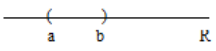
Open interval (a,b) = {x ∈ R: a < x < b} It is geometrically represented by

Left open interval
(a, b] = {x ∈ R: a < x ≤ b}. It is geometrically represented by

Right open interval
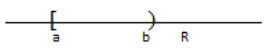
[a, b) = {x ∈ R: a ≤ x < b}. It is geometrically represented by

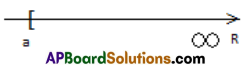
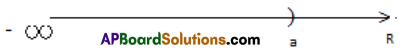
[a, ∞) = {x ∈ R : x ≥ a} = {x ∈ R : a ≤ x < ∞} It is geometrically represented by

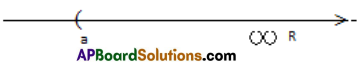
(a, ∞) = {x ∈ R : x > a} = {x ∈ R : a < x < ∞}

(-∞, a] = {x ∈ R : x ≤ a} = {xe R : -∞ < x < a}

Neighbourhood of A Point: Definition: Let ae R. If δ > 0 then the open interval (a – δ, a + δ) is called the neighbourhood (δ – nbd) of the point a. It is denoted by N_δ (a) . a is called the centre and δ is called the radius of the neighbourhood .
∴ N_δ(a) = (a – δ, a + δ) = {x ∈ R: a – δ< x < a + δ} = {x ∈ R: |x – a| < δ}

The set N_δ(a) – {a} is called a deleted δ – neighbourhood of the point a.
∴ N_δ(a) – {a} = (a – δ, a) ∪ (a, a + δ) = {x ∈ R :0 < | x – a | < δ}
Note: (a – δ, a) is called left δ -neighbourhood, (a, a + δ) is called right δ – neighbourhood of a

Graph of A Function:

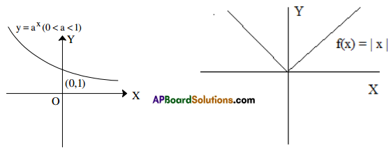
Mod function:
The function f: R-R defined by f(x) = |x| is called the mod function or modulus function or absolute value function.
Dom f R. Range f [0, )

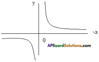
Reciprocal function :
The function f: R – {0} – R defined by
f(x) = \(\frac{1}{x}\) is called the reciprocal function,
Dom f = R – {0}= Range f = R

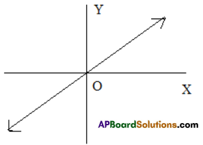
Identity function:
The function f R-R defined by f(x) = x is called the identity
It is denoted by I(x)

Limit of A Function
Concept of limit:
Before giving the formal definition of limit consider the following example.
Let f be a function defined by f (x) = \(\frac{x^{2}-4}{x-2}\). clearly, f is not defined at x = 2.
When x ≠ 2, x – 2 ≠ 0 and f(x) = \(\frac{(x-2)(x+2)}{x-2}\) = x + 2

Now consider the values of f(x) when x ≠ 2, but very very close to 2 and <2.

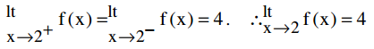
It is clear from the above table that as x approaches 2 i.e.,x → 2 through the values less than 2, the value of f(x) approaches 4 i.e., f(x) → 4. We will express this fact by saying that left hand limit of f(x) as x → -2 exists and is equal to 4 and in symbols we shall write \({lt}_{x \rightarrow 2^{-}} f(x)\) = 4

Again we consider the values of f(x) when x ≠ 2, but is very-very close to 2 and x > 2.

It is clear from the above table that as x approaches 2 i.e.,x → 2 through the values greater than 2, the value of f(x) approaches 4 i.e., f(x) → 4. We will express this fact by saying that right hand
limit of f(x) as x → 2 exists and is equal to 4 and in symbols we shall write \({lt}_{x \rightarrow 2^{+}} f(x)\) = 4

Thus we see that f(x) is not defined at x = 2 but its left hand and right hand limits as x → 2 exist and are equal.
When \({lt}_{\mathrm{x} \rightarrow \mathrm{a}^{+}} \mathrm{f}(\mathrm{x}), \mathrm{lt}_{\mathrm{x} \rightarrow \mathrm{a}^{-}}^{\mathrm{f}(\mathrm{x})}\) are equal to the same number l, we say that \(\begin{array}{ll}
l_{x \rightarrow a} & f(x)
\end{array}\) exist and equal to 1.

Thus, in above example,

One Sided Limits Definition Of Left Hand Limit:
Let f be a function defined on (a – h, a), h > 0. A number l1 is said to be the left hand limit (LHL) or left limit (LL) of f at a if to each
ε >0, ∃ a δ >0 such that, a – δ < x < a ⇒ |f (x) – l₁| < ε.
In this case we write \(\underset{x \rightarrow a-}{L t} f(x)\) = l₁ (or) \({Lt}_{x \rightarrow a-0} f(x)\) = l₁

Definition of Right Limit:
Let f be a function defined on (a, a + h), h > 0. A number l ₂is said to the right hand limit (RHL) or right limit (RL) of f at a if to each ε >0, ∃ a δ >0 such that, a – δ < x < a ⇒ |f (x) – l₂| < ε.
In this case we write \(\underset{x \rightarrow a+}{L t} f(x)\) = l₂ (or) \({Lt}_{x \rightarrow a+0} f(x)\) = l₂

Definition of Limit:
Let A ∈ R, a be a limit point of A and
f : A → R. A real number l is said to be the limit of f at a if to each ε > 0, ∃ a δ > 0 such that x ∈ A, 0 < |x – a| < δ ⇒ | f(x) – l| < ε. In this case we write f (x) → 2 (or) \({Lt}_{x \rightarrow a} f(x)\) = l. Note: 1.If a function f is defined on (a – h, a) for some h > 0 and is not defined on (a, a + h) and if \(\underset{x \rightarrow a-}{{Lt}} f(x)\) exists then \({Lt}_{x \rightarrow a} f(x)={Lt}_{x \rightarrow a-} f(x)\).
2. If a function f is defined on (a, a + h) for some h > 0 and is not defined on (a – h, a) and if \(\underset{x \rightarrow a+}{{Lt}} f(x)\) exists then \({Lt}_{x \rightarrow a} f(x)={Lt}_{x \rightarrow a+} f(x)\).

Theorem:
If \({Lt}_{x \rightarrow a} f(x)\) exists then \({Lt}_{x \rightarrow a} f(x)={Lt}_{x \rightarrow 0} f(x+a)={Lt}_{x \rightarrow 0} f(a-x)\)

Theorems on Limits WithOut Proofs
1. If f : R → R defined by f(x) = c, a constant then \({Lt}_{x \rightarrow a} f(x)\) = c for any a ∈ R.

2. If f: R → R defined by f(x) = x, then \({Lt}_{x \rightarrow a} f(x)\) = a i.e., \({Lt}_{x \rightarrow a} f(x)\) = a (a ∈ R)

3. Algebra of limits

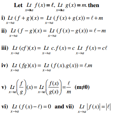
vii) If f(x) ≤ g(x) in some deleted neighbourhood of a, then \({Lt}_{x \rightarrow a} f(x) \leq {Lt}_{x \rightarrow a} g(x)\)
viii) If f(x) ≤ h(x) < g(x) in a deleted nbd of a and \({Lt}_{x \rightarrow a} f(x)\) = l = \({Lt}_{x \rightarrow a} g(x)\) then \({Lt}_{x \rightarrow a} h(x)\) = l
ix) If \({Lt}_{x \rightarrow a} f(x)\) = 0 and g(x) is a bounded function in a deleted nbd of a then \({Lt}_{x \rightarrow a}\) f(x) g(x) = 0.

Theorem
If n is a positive integer then \({Lt}_{x \rightarrow a} x^{n}\) = aⁿ, a ∈ R

Theorem
If f(x) is a polynomial function, then \({Lt}_{x \rightarrow a}\)f(x) = f (a)

Evaluation of Limits:
Evaluation of limits involving algebraic functions.
To evaluate the limits involving algebraic functions we use the following methods:

• Direct substitution method
• Factorisation method
• Rationalisation method
• Application of the standard limits.

1. Direct substitution method:
This method can be used in the following cases:

• If f(x) is a polynomial function, then \({Lt}_{x \rightarrow a}\)f(x) = f (a).
• If f (x) = \(\frac{P(a)}{Q(a)}\) where P(x) and Q(x) are polynomial functions then \({Lt}_{x \rightarrow a}\)f(x) = \(\frac{P(a)}{Q(a)}\) provided Q(a) ≠ 0.

2. Factiorisation Method:
This method is used when \({Lt}_{x \rightarrow a}\)f (x) is taking the indeterminate form of the type 0 by the substitution of x = a.
In such a case the numerator (Nr.) and the denominator (Dr.) are factorized and the common factor (x – a) is cancelled. After eliminating the common factor the substitution x = a gives the limit, if it exists.

3. Rationalisation Method : This method is used when \({Lt}_{x \rightarrow a} \frac{f(x)}{g(x)}\) is a \(\frac{0}{0}\) form and either the Nr. or Dr. consists of expressions involving radical signs.

4. Application of the standard limits.
In order to evaluate the given limits , we reduce the given limits into standard limits form and then we apply the standard limits.

Theorem 1.
If n is a rational number and a > 0 then \({Lt}_{x \rightarrow a} \frac{x^{n}-a^{n}}{x-a}\) = n.a^n-1

Note:

• If n is a positive integer, then for any a ∈ R. \({Lt}_{x \rightarrow a} \frac{x^{n}-a^{n}}{x-a}\) = n.a^n-1
• If n is a real number and a> 0 then \({Lt}_{x \rightarrow a} \frac{x^{n}-a^{n}}{x-a}\) = n.a^n-1
• If m and n are any real numbers and a > 0, then \({Lt}_{x \rightarrow a} \frac{x^{m}-a^{m}}{x^{n}-a^{n}}=\frac{m}{n}\)a^m-n

Theorem 2.
If 0 < x < \(\frac{\pi}{2}\) then sin x < x < tan x.

Corollary 1:
If – \(\frac{\pi}{2}\) < x < 0 then tan x < x < sin x

Corollary 2:
If 0 < |x| < \(\frac{\pi}{2}\) then |sin x| < |x| < |tan x|

Standard Limits:

• \({Lt}_{x \rightarrow 0} \frac{\sin x}{x}\) = 1
• \(\underset{x \rightarrow 0}{L t} \frac{\tan x}{x}\) = 1
• \({Lt}_{x \rightarrow 0} \frac{e^{x}-1}{x}\) = 1
• \({Lt}_{x \rightarrow 0} \frac{a^{x}-1}{x}\) = log_ea
• \({Lt}_{x \rightarrow 0}(1+x)^{\frac{1}{x}}\) = e
• \({Lt}_{x \rightarrow \infty}\left(1+\frac{1}{x}\right)^{x}\) = e
• \({Lt}_{x \rightarrow \infty}\left(1+\frac{1}{x}\right)^{x}\) = e

Limits At Infinity
Definition:
Let f(x) be a function defined on A = (K,).
(i) A real number l is said to be the limit of f(x) at ∞ if to each δ > 0, ∃ , an M > 0 (however large M may be) such that x ∈ A and x > M ⇒ |f (x) – l|< δ.
In this case we write f (x) → l as x → +∞ or \({Lt}_{x \rightarrow \infty} f(x)\) = l.

(ii) A real number l is said to be the limit of f(x) at -∞ if to each δ > 0, ∃ > 0, an M > 0 (however large it may be) such that x ∈ A and x < – M ⇒ |f (x) – l| < δ. In this case, we write f (x) → l as x → -∞ or \({Lt}_{x \rightarrow \infty} f(x)\) = l.

Infinite Limits Definition:
(i) Let f be a function defined is a deleted neighbourhood of D of a. (i) The limit of f at a is said to be ∞ if to each M > 0 (however large it may be) a δ > 0 such that x ∈ D, 0 < |x – a| < δ ⇒ f(x) > M. In this case we write f(x) as x → a or \({Lt}_{x \rightarrow a} f(x)\) = +∞

(ii) The limit of f(x) at a is said be -∞ if to each M > 0 (however large it may be) a δ > 0 such that x ∈ D, 0 < | x – a | < δ ⇒ f(x) < – M. In thise case we write f(x) → -∞ as x → a or \({Lt}_{x \rightarrow a} f(x)\) = -∞

Indeterminate Forms:
While evaluation limits of functions, we often get forms of the type \(\frac{0}{0}, \frac{\infty}{\infty}\), 0 × -∞, 0⁰, 1^∞, ∞⁰ which are termed as indeterminate forms.

Continuity At A Point:
Let f be a function defined in a neighbourhood of a point a. Then f is said to be continuous at the point a if and only if \({Lt}_{x \rightarrow a} f(x)\) = f (a).
In other words, f is continuous at a iff the limit of f at a is equal to the value of f at a.

Note:

• If f is not continuous at a it is said to be discontinuous at a, and a is called a point of discontinuity of f.
• Let f be a function defined in a nbd of a point a. Then f is said to be
  • Left continuous at a iff \({Lt}_{x \rightarrow a-} f(x)\) = f (a).
  • Right continuous at a iff \({Lt}_{x \rightarrow a+} f(x)\) = f (a).
• f is continuous at a iff f is both left continuous and right continuous at a
  i.e, \({Lt}_{x \rightarrow a} f(x)=f(a) \Leftrightarrow {Lt}_{x \rightarrow a^{-}} f(x)=f(a)={Lt}_{x \rightarrow a+} f(x)\)

Continuity of A Function Over An Interval:
A function f defined on (a, b) is said to be continuous (a,b) if it is continuous at everypoint of (a, b) i.e., if \({Lt}_{x \rightarrow c} f(x)\) =f (c) ∀c ∈ (a, b)
II) A function f defined on [a, b] is said to be continuous on [a, b] if

• f is continuous on (a, b) i.e., \({Lt}_{x \rightarrow c} f(x)\) = f (c) ∀c ∈(a, b)
• f is right continuous at a i.e., \({Lt}_{x \rightarrow a+} f(x)\) = f (a)
• f is left continuous at b i.e., \({Lt}_{x \rightarrow b-} f(x)\) = f (b).

Note :

• Let the functions f and g be continuous at a and k€R. Then f + g, f – g, kf , kf + lg, f.g are continuous at a and \(\frac{f}{g}\) is continuous at a provided g(a) ≠ 0.
• All trigonometric functions, Inverse trigonometric functions, hyperbolic functions and inverse hyperbolic functions are continuous in their domains of definition.
• A constant function is continuous on R
• The identity function is continuous on R.
• Every polynomial function is continuous on R.